Assembly Variant Finder identifies variants in a project genome relative to a closely related reference genome. It combines variant calling, predicted effects, and interactive sequence browsing in one report.

• Find single-nucleotide variants, insertions, and deletions in assembled bacterial genomes.
• Locate changes on a reference sequence and interpret them using its gene annotation.
• Search and filter calls, inspect every predicted consequence, and browse the complete reference contigs.
• Download variant files, consequence tables, callable regions, and figures for further analysis.

The two genomes have distinct roles. The project genome is the sample under investigation, such as a newly sequenced isolate. The reference genome is the baseline against which its variants are called. Variant positions, reference alleles, gene annotations, and the sequence in the viewer all belong to the reference. An insertion represents sequence added in the project relative to the reference; a deletion represents reference sequence absent from the project.

The tool aligns the project to the reference with minimap2, described in Heng Li's paper Minimap2: pairwise alignment for nucleotide sequences, and calls variants with paftools.js. An annotated reference in GenBank format, or reference FASTA plus GFF3, enables SnpEff predictions against the reference's genes and transcripts. The SnpEff method is described by Cingolani and colleagues. A reference without annotation still supports variant calling and sequence browsing.

When optional automatic preset selection is enabled, the tool uses an initial alignment to choose the alignment setting and records its choice in the report. Explicit manual presets remain available.

Poorly aligned regions can leave differences between genomes undetected. The report therefore shows how much of the reference could be assessed and explains any coverage or similarity limitations. If too little sequence can be compared, or the genomes exceed the supported divergence threshold, it provides an assessment without a final variant list.

The example below compares Escherichia coli K-12 W3110 as the project (AP009048.1) with MG1655 as the reference (NC_000913.3). The interactive report presents the variants in a table, with one row for each difference and columns for its reference position, type, gene, and primary predicted consequence. Selecting a variant's row updates the details panel beside the table. Its Overview tab shows the sequence change and supporting alignment evidence; the Consequences tab provides the full set of gene and transcript predictions for that variant.

At the highlighted position in `dgcT`, W3110 has T where the MG1655 reference has C (reference position 1,093,264). Relative to alanine at position 130 of the MG1655 reference protein, SnpEff predicts valine at the corresponding position in W3110, the project strain. This change is shown as p.Ala130Val in the details panel.

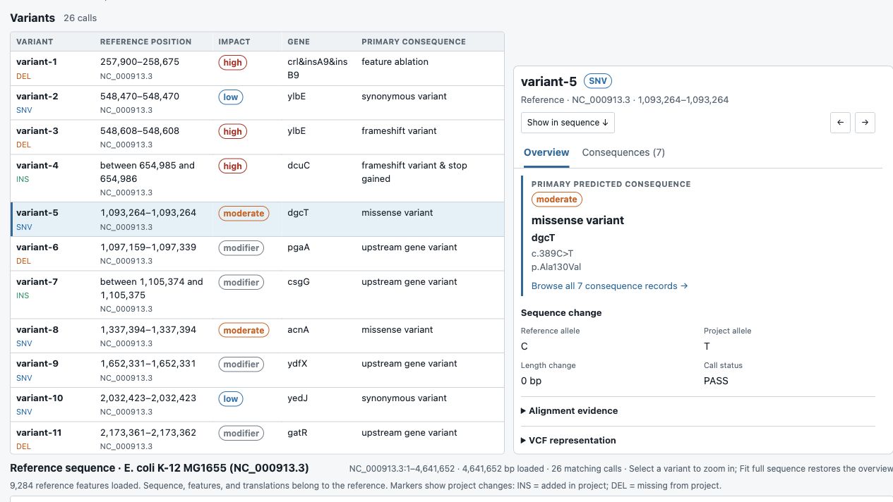
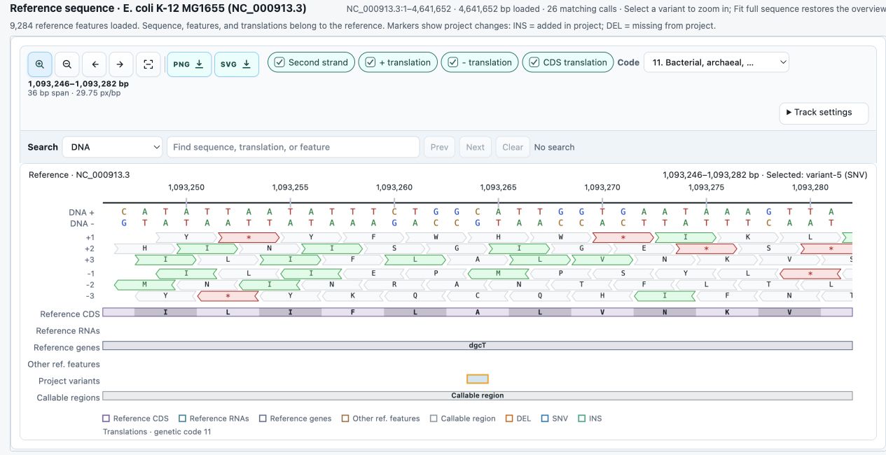
The interactive report supports searching the variant table by gene, predicted consequence, or reference position, and filtering by variant type or predicted impact. For a closer look, Show in sequence opens the selected variant's surroundings in a viewer derived from Sequence Manipulation Suite 3. The compact viewer places DNA above translations and annotation tracks. At close zoom, the CDS translation option displays amino-acid letters inside annotated coding regions, with each letter aligned to its reference codon. Individual DNA bases and translations can be inspected, the sequence can be searched, and the view can be zoomed out to explore larger regions or the whole reference contig. The viewer and details panel stay linked as different variants are selected. Feature hover cards expose annotation notes and other qualifiers, including pseudogene flags, to help explain features whose names alone are not informative.

The highlighted box marks the same `dgcT` variant on the MG1655 reference sequence. The two reference DNA strands appear above their six reading-frame translations, with arrows indicating translation direction. The ruler gives positions along the reference chromosome; annotation and variant tracks appear below the translations. The Reference CDS row shows the annotated `dgcT` protein, including alanine (A) at the highlighted codon.

The analysis also produces downloadable files for follow-up work:

• Variant VCF files record each change's reference position and reference and project alleles for use with other variant-analysis tools.
• Variant tables in TSV, downloadable from the interactive report, list positions, sequence changes, and supporting details for spreadsheet review or analysis scripts.
• Consequence tables in TSV and JSON, downloadable from the report when reference annotation is supplied, link each matching variant to its gene and transcript annotations and predicted DNA and protein changes. They include every reported consequence for each matching variant.
• Callable-region BED files identify the reference intervals that met the alignment and coverage requirements for variant calling. These intervals distinguish assessed regions from those where differences could have gone undetected.

Report table downloads follow the current display filters and include matching calls beyond the visible page. To export the entire callset, select All calls and All contigs, and clear the other filters. The complete VCF retains both PASS and non-PASS calls. In compact output, VCF and BED downloads are compressed and supplied with matching indexes; tables remain available through the report, while separate calls JSON and duplicate table files are omitted.

The current sequence view can be exported as a PNG or SVG figure. The downloadable HTML report supports offline browsing of the results and reference sequence.

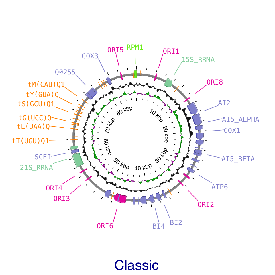
Proksee’s updated label system gives you more control over how feature labels appear on your maps. Choose between Classic and Adaptive placement, adjust label density, and access the main settings through a new popup beside your map.

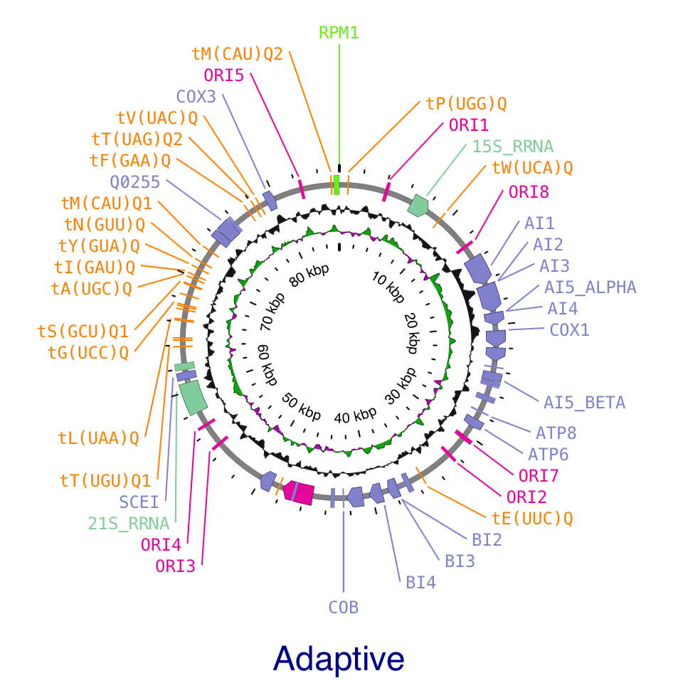
Adaptive adjusts label placement to the density of features and the available space. At low density, labels follow an oval around a full circular map. As density increases, crowded regions reorganize to fit more labels while less crowded regions can retain a simpler arrangement. Smooth transitions during panning and zooming make labels easier to follow as their positions change.

Classic uses straight leader lines and arranges labels in outward levels, providing a familiar layout for both circular and linear maps.

Both methods share a Density slider. Move toward Low for a cleaner layout or toward High to display more labels. You can also keep labels within the visible map area and adjust their spacing, font size, and leader line width.

Click the gear beneath the label visibility button to open the new settings popup. It provides quick access to the main label controls and shows the total number of labels and the number currently drawn. Click the Labels title to open the full settings in the sidebar.

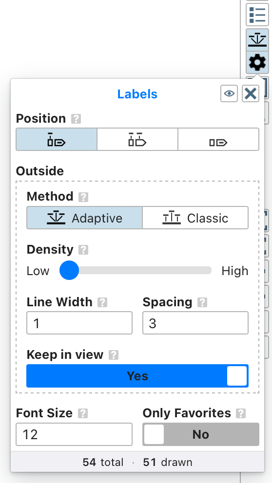
Existing maps are updated automatically when opened: Default placement becomes Classic, and Angled placement becomes Adaptive. Adaptive is the default for new maps, and you can switch between the two methods at any time.

A new tool has been added to Proksee:

Genome Identity Matrix

• Compare two or more complete or draft microbial genome assemblies with FastANI.
• Explore directional average nucleotide identity (ANI), distance, and alignment-fraction matrices.
• Group similar genomes with average-linkage clustering and matching dendrograms.
• Inspect FastANI fragment mappings for individual query–reference comparisons.
• Download matrix tables, figures, pairwise views, and summary metadata for downstream review.

FastANI was developed by Chirag Jain and colleagues for fast, whole-genome ANI estimation. The method and its large-scale application are described in their Nature Communications paper, High throughput ANI analysis of 90K prokaryotic genomes reveals clear species boundaries.

Genome Identity Matrix packages all directional FastANI comparisons into one interactive report. Users can switch among ANI, distance, and alignment fraction; view genomes in input or clustered order; add dendrograms; search genome labels; and inspect exact values for each query–reference cell. The displayed matrix can be exported as SVG, PNG, or ordered CSV.

The examples below use the tool's five-genome diagnostic data set. The 600 kb assembly, close_a, and close_b genomes produce dense collinear mappings. The 600 kb rearranged genome retains sixteen 30 kb blocks in a changed order, mixes in four unrelated blocks, and is stored as twenty FASTA records. The distant genome provides comparisons for which FastANI reports no value.

The clustered ANI view groups the related genomes while leaving the deliberately distant genome separated. Gray `NA` cells mean that FastANI did not report a value; they do not represent zero similarity.

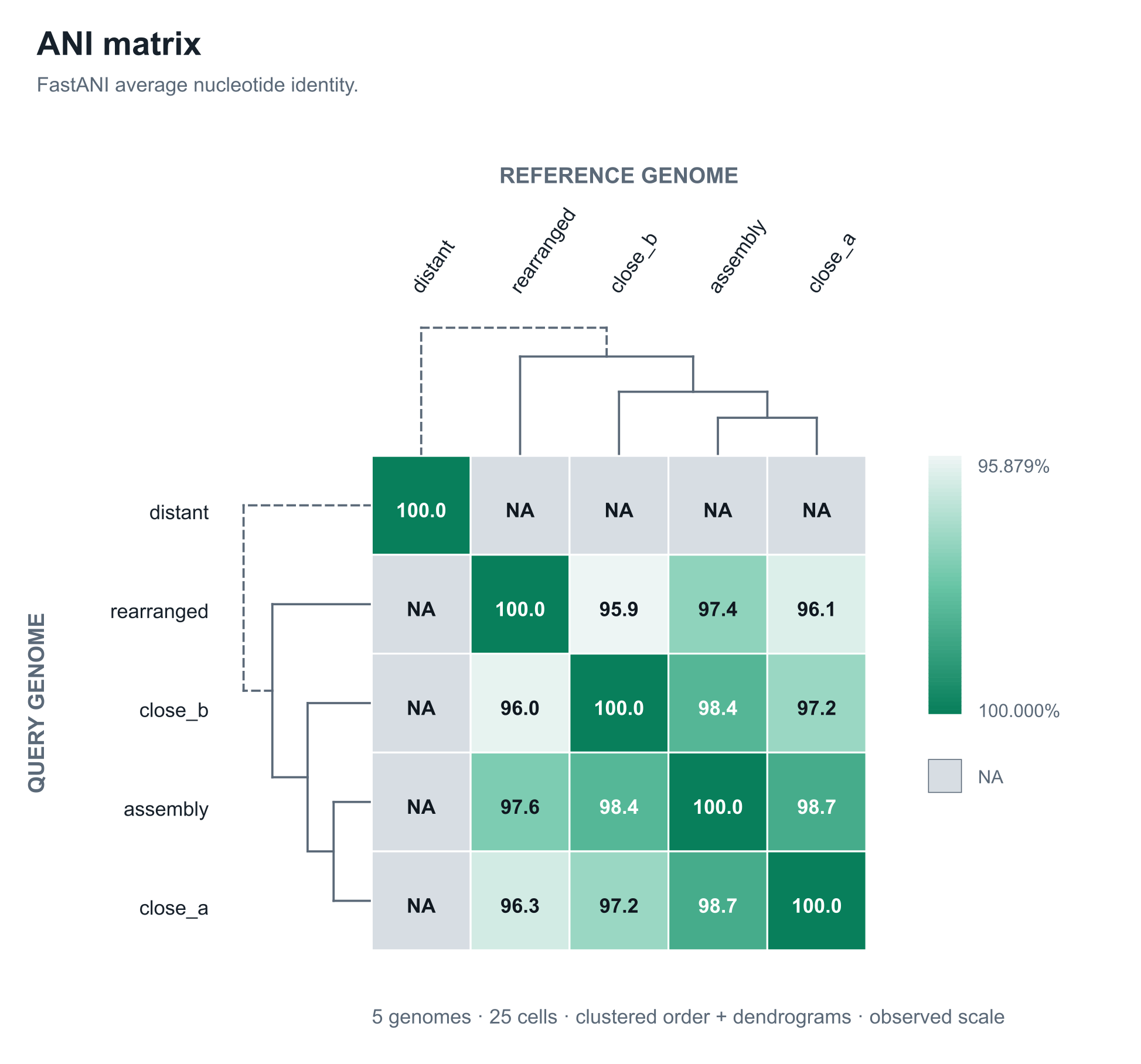
The dendrograms use average-linkage clustering on 100 − ANI, combining available results from both comparison directions. Solid joins are supported by FastANI distances; dashed joins indicate that no FastANI value was available between the connected clusters.

Selecting a matrix cell opens its directional FastANI fragment-mapping view. The reference genome is shown on top and the query genome below on one shared base-pair scale. A reference-position colour is copied to each linked query block, so smooth colour order supports conserved placement while reordered colours and crossing ribbons reveal changed sequence order or placement. Uncoloured intervals lack a plotted FastANI mapping, and darker ribbons represent higher fragment identity.

The diagnostic `assembly` query versus `rearranged` reference comparison has 97.624% ANI, a 67.50% alignment fraction, and 135 fragment mappings. Crossing ribbons and reordered colours show that mapped fragments occur in different relative positions between the two genomes, while gaps mark intervals without a plotted FastANI mapping.

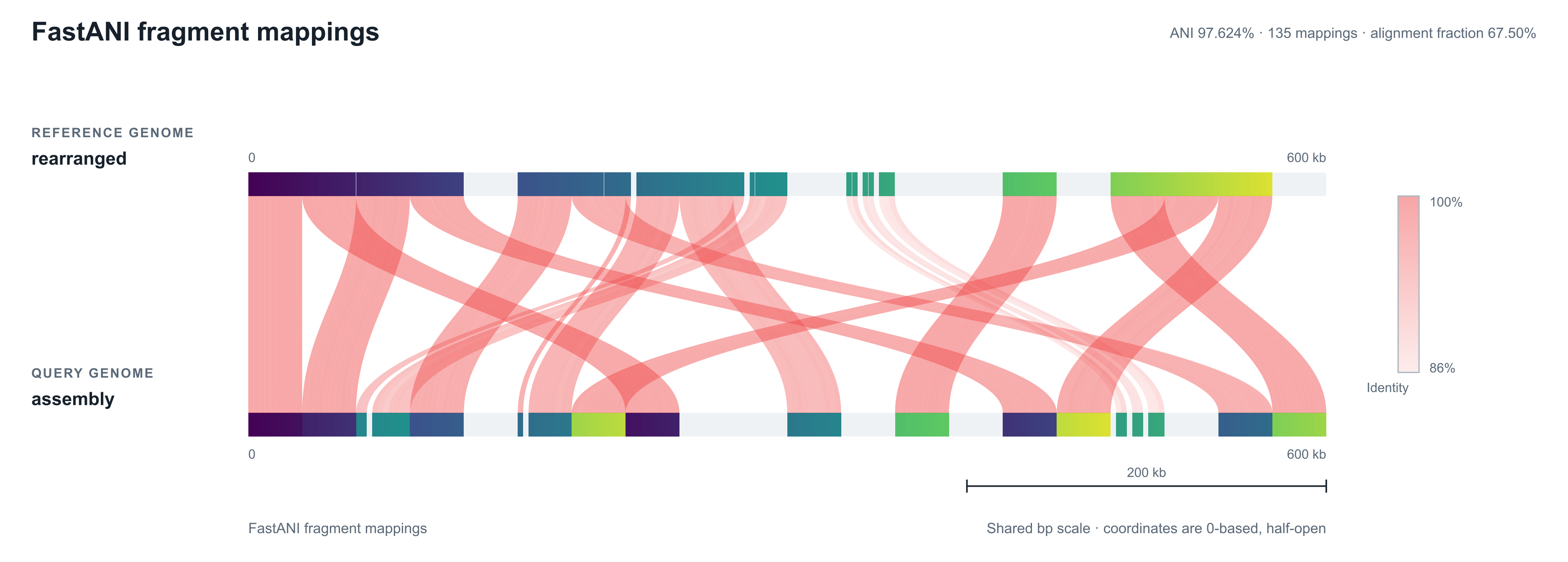
Genome Identity Matrix runs FastANI separately in both directions for every genome pair. The two results remain visible in opposite matrix cells and in separate pairwise views; the displayed ANI and alignment fraction values are not averaged. Because alignment fraction is calculated relative to the query genome, the two directions can differ. Fragmented-assembly record order can also create rearrangement-like mapping patterns, and FastANI's visual output does not report strand, so unexpected patterns are best followed with more detailed analysis.

Proksee’s latest map-viewer update brings six-frame translation, richer sequence detail, and new feature and track labels. Powered by CGView 1.9, these additions make it easier to explore your genome at different scales.

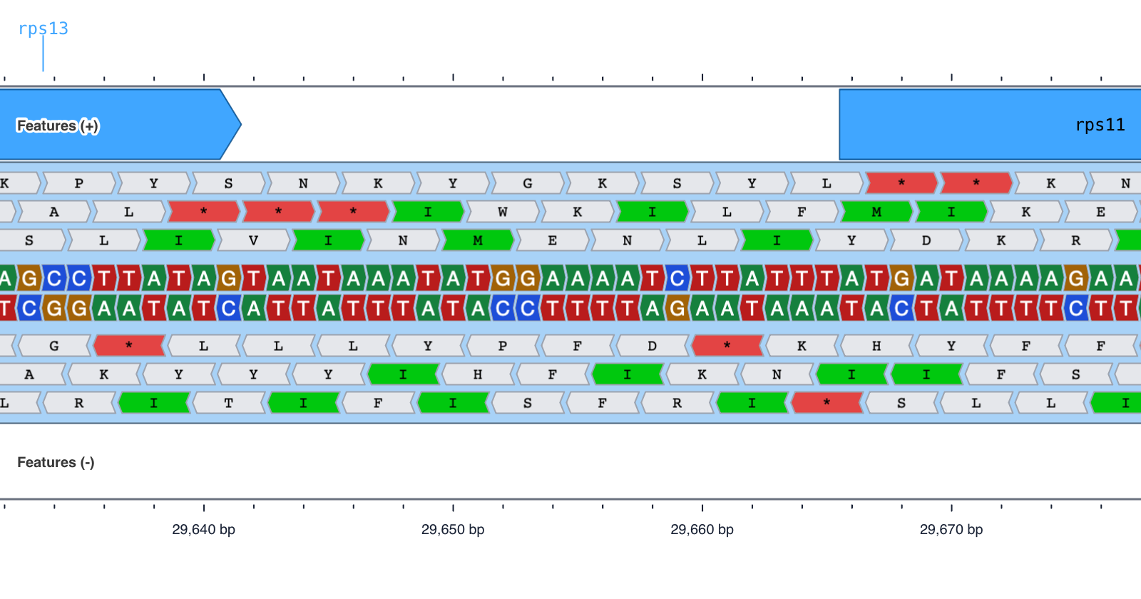
• Explore all six reading frames. Zoom into the nucleotide sequence to see amino-acid translations on both strands, with start and stop codons highlighted. Hover over a translated codon to inspect its amino acid, sequence, position, reading frame, and genetic code.
• See more sequence detail. Distinct nucleotide colors and directional boxes make individual bases easier to distinguish. Choose colored boxes, uniform boxes, or letters only, with horizontal text or text that follows a circular map.

Zooming in reveals individual bases and amino-acid translations in all six reading frames, with start codons highlighted in green and stop codons in red.

• Read feature names directly on the map. Inline labels place names inside their features. Auto placement uses inline labels where they fit and falls back to outside placement. Optional shrinking and truncation provide additional control.
• Identify tracks as you zoom in. Labels identify each track and its individual slots, helping you stay oriented while exploring a region.

Inline labels place names inside features. Track labels identify each track and its individual slots, including strand, reading-frame, type, or legend details where applicable.

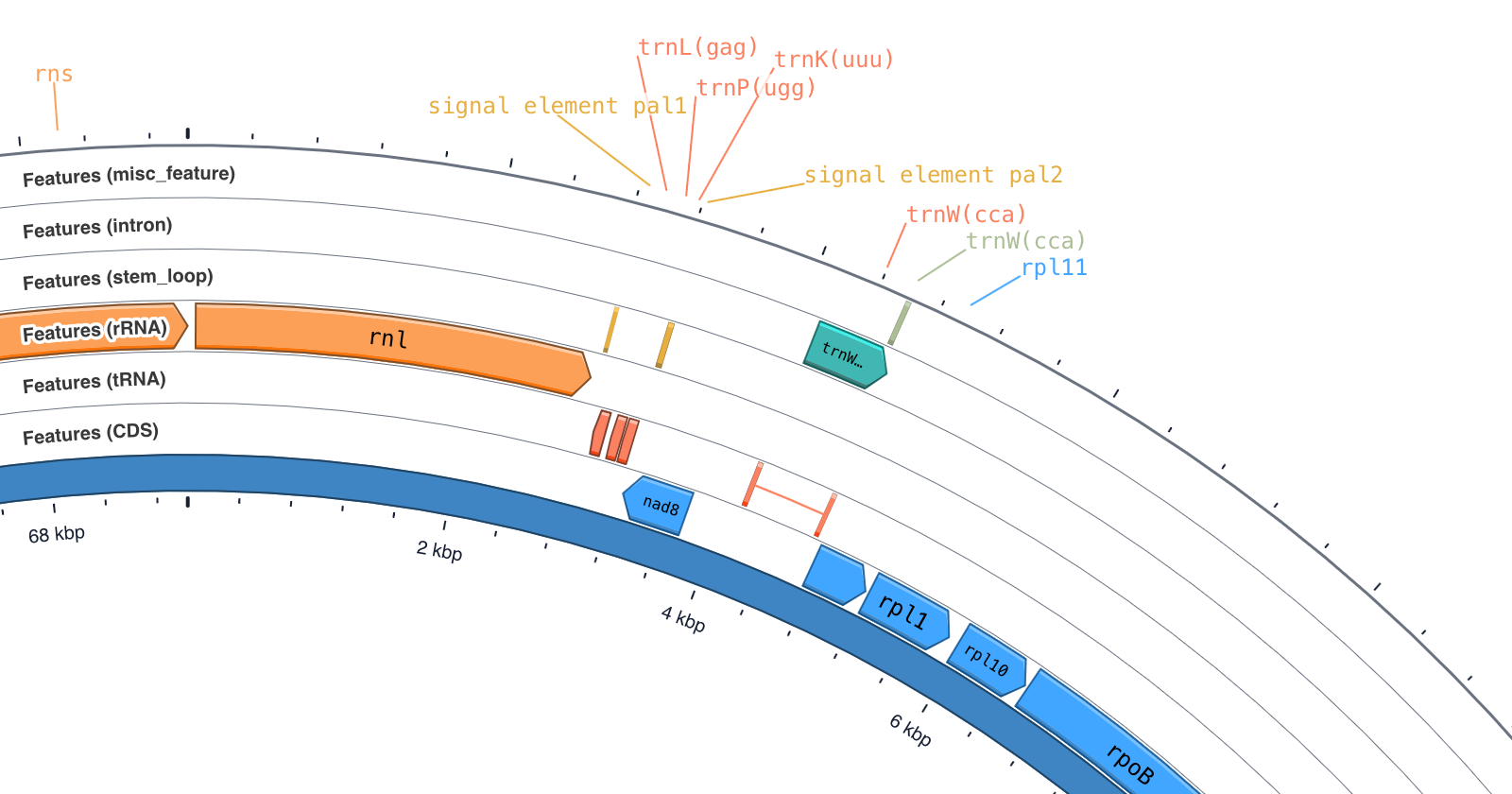
• Let feature arrows adapt to zoom. The new Auto option displays features as arcs when they are small on screen and progressively reveals arrowheads as you zoom in.
• Adjust track thickness more precisely. Fine-tune the width of track slots using relative ratios or pixel values.
• Choose where ruler labels appear. Place coordinate labels inside, outside, or on both sides of the map, or hide them. Circular maps also support labels that follow the curve.

The update also improves the contours of line plots such as GC content and GC skew, and fixes blurry arcs when viewing zoomed circular maps in Safari. Proksee now remembers your selected sidebar tabs between visits.

Proksee’s genome assembly functionality has been completely rewritten. The new Assembly Tool can assemble genomes directly from short and long sequencing reads.

The new Assembly Tool supports three types of assembly:

• Short-read assembly using SKESA, MEGAHIT, or SPAdes
• Long-read assembly using Flye
• Hybrid assembly from combined short and long reads using Unicycler

Users can upload raw FASTQ files and go directly from sequencing reads to an assembled genome and interactive Proksee map.

The tool also includes a comprehensive quality-control workflow. Reads are filtered and assessed before assembly, and the resulting assembly is evaluated using a range of post-assembly analyses. These include standard analyses of genome completeness, contamination, and taxonomy, as well as new approaches to k-mer completeness and contig binning.

Each analysis produces a detailed Assembly Report containing the results, figures, software and database versions, workflow settings, and checksums for the input files and final assembly. The report is designed to provide both an overview of assembly quality and the information needed to understand and reproduce the analysis.

Once assembly is complete, the assembled contigs are loaded directly into Proksee, where they can be annotated, analyzed, and visualized using Proksee’s existing tools.

The Assembly Tool is currently in beta. We welcome feedback as we continue to improve the workflow.